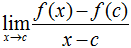
So far we have looked at derivatives outside of the notion of differentiability. The problem with this approach, though, is that some functions have one or many points or intervals where their derivatives are undefined. A function f is differentiable at a point c if
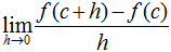 exists.
Similarly, f is differentiable on an open interval (a, b) if
exists for every c in (a, b).
Basically, f is differentiable at c if f'(c) is defined, by the above definition. Another point of note is that if f is differentiable at c, then f is continuous at c.
Let's go through a few examples and discuss their differentiability. First, consider the following function.
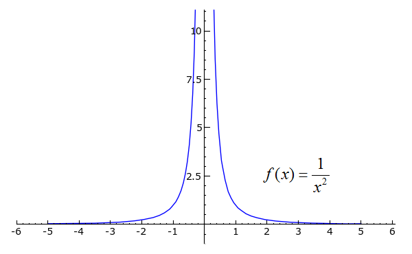
plot(1/x^2, x, -5, 5).show(ymin=0, ymax=10)Toggle Line Numbers
To find the limit of the function's slope when the change in x is 0, we can either use the true definition of the derivative and do
def f(x):
    return 1/x^2

var('h')
((f(x+h)-f(x))/h).rational_simplify().subs(h=0)
Toggle Line Numbers
or we can simply use the rules of differentiation by calling 'derivative(1/x^2, x)'. In any case, we find that
Since f'(x) is undefined when x = 0 (-2/02 = ?), we say that f is not differentiable at x = 0. Since f'(x) is defined for every other x, we can say that f' is continuous on (-∞, 0) U (0, ∞), where "U" denotes the union of two intervals.
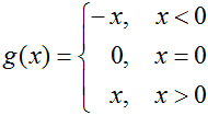
How about a function that is everywhere continuous but is not everywhere differentiable? This occurs quite often with piecewise functions, since even though two intervals might be connected, the slope can change radically at their junction. Take a look at the function g(x) = |x|.
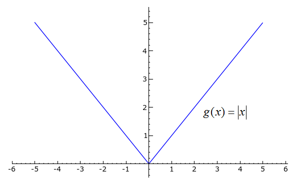
plot(abs(x), x, -5, 5)Toggle Explanation Toggle Line Numbers
1) Plot the absolute value of x from -5 to 5.
Using our knowledge of what "absolute value" means, we can rewrite g(x) in the expanded form
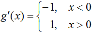
This should be easy to differentiate now; we get
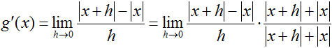
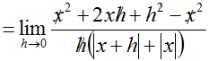
What about at x = 0? The "logical" response would be to see that g(0) = 0 and say that g'(0) must therefore equal 0. Careful, though...looking back at the limit definition of the derivative, the derivative of f at a point c is the limit of the slope of f as the change in its independent variable approaches 0. Really, the only relevant piece of information is the behavior of function's slope close to c. Referring back to the example, since the limit of g'(x) as x approaches 0 from the left ≠ the limit of g'(x) as x approaches 0 from the right, g'(0) does not exist. We can use the limit definition of the derivative to prove this:
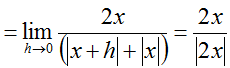
 ,
so
,
so  ,
which is undefined.
,
which is undefined.
In this form, it makes far more sense why g'(0) is undefined. By simply looking at the graph of g, too, one can see that the sudden "twist" at x = 0 is responsible for our inability to evaluate g' there. We can now justly pronounce that g is differentiable on (-∞, 0) U (0, ∞), so g' is continuous on that same interval.
The third function of discussion has a couple of quirks--take a look.
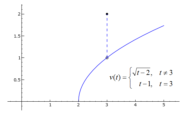
p = plot(sqrt(x-2), x, 2, 5)
pt1 = point((3, 1), rgbcolor="white", pointsize=30, faceted=True)
pt2 = point((3, 2), rgbcolor="black", pointsize=30)
l = line([(3, 1), (3, 2)], linestyle="--")
(p+pt1+pt2+l).show(xmin=0)
Toggle Line Numbers
Not only is v(t) defined solely on [2, ∞), it has a jump discontinuity at t = 3. The jump discontinuity causes v'(t) to be undefined at t = 3; do you see why? Using a slightly modified limit definition of the derivative, think of what
would be for c = 3 and some x very close to 3. The resulting slope would be astronomically large either negatively or positively, right? In fact, the dashed line connecting v(t) for t ≠ 3 and v(3) is what the tangent line will look like at that point. Since a function's derivative cannot be infinitely large and still be considered to "exist" at that point, v is not differentiable at t=3.
The Mean Value Theorem is very important for the discussion of derivatives; even though it might seem somewhat obvious, it is actually very important to many other concepts in calculus. We'll start with an example.
Consider the vast, seemingly endless state of Montana. Now, pretend that you are driving across Montana so that you can get to Washington, and you want to do so as quickly as possible. The problem, however, is that the signs posted every few miles explicitly state that the speed limit is 70 miles per hour. "Oh well," you tell yourself. "When I'm on the open road, I will go as fast as I want. When I approach a town, though, I will slow down so that the police are none the wiser."
Since you had been staying with some relatives in the town of Springdale, you first head east at the brisk pace of 90 miles per hour until, feeling your stomach rumble (you really aren't cut out for these long drives), you stop in Livingston for some lunch. When you arrive, however, a policeman signals you to pull over! "What did I do wrong?" you sweetly ask the officer. Giving you a hard look, the policeman responds, "Though I didn't actually see you speeding at any point on your way here, I know that you must have, since one of my buddies back in Livingston tells me that you left there only 10 minutes ago, and our two towns are about 15 miles apart. I won't cite you for it this time, but you'd better drive slower in the future."
The question is: How did the policeman know you had been speeding? Well, since it took you 10 minutes to travel 15 miles, your average speed was 90 miles per hour. So either you traveled at exactly 90 miles per hour the entire time, or you traveled at more than 90 part of the way and less than ninety part of the way. In either case, you were going faster than the speed limit at some point in time.
The Mean Value Theorem has a very similar message: if a function f is continuous on the closed interval [a, b] and is differentiable on the open interval (a, b), then there is some c in (a, b) such that
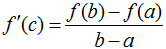
Basically, the average slope of f between a and b will equal the actual slope of f at some point between a and b. To illustrate the Mean Value Theorem, consider the function f(x) = x*sin(x) for x in [0, 9π/2]. Assume that f is differentiable on (0, 9π/2) (it is) and continuous on [0, 9π/2] (it is). By the Mean Value Theorem, there is at least one c in (0, 9π/2) such that
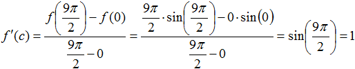 .
.
And such a c does exist, in fact. You can use SageMath's solve function to verify this:
solve(derivative(x*sin(x), x) == 0, x)Toggle Line Numbers
From the code's output, you can see that this is true whenever -sin(x)/cos(x) is 0. Thus c = 0, π, 2π, 3π, and 4π, so the Mean Value Theorem is satisfied for f on the interval [0, 9π/2].
Rolle's Theorem states that if a function g is differentiable on (a, b), continuous [a, b], and g(a) = g(b), then there is at least one number c in (a, b) such that g'(c) = 0. To see this, consider the everywhere differentiable and everywhere continuous function g(x) = (x-3)*(x+2)*(x^2+4). To prove that g' has at least one zero for x in (-∞, ∞), notice that g(3) = g(-2) = 0. By Rolle's Theorem, there must be at least one c in (-2, 3) such that g'(c) = 0.
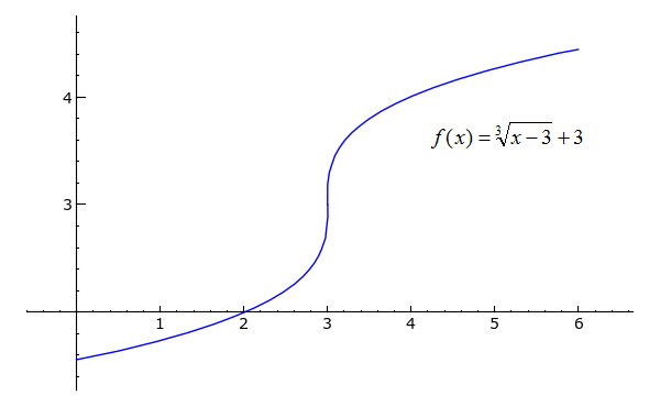
plot((x-3)^(1/3)+3, x, 3, 6) + plot(-(-x+3)^(1/3)+3, x, 0, 3)Toggle Explanation Toggle Line Numbers
1) Taking the cube root (or any odd root) of a negative number does not work well in Python, so one has to use multiple plot commands for functions such as x^(1/3) to compensate for the intervals on which x is negative.
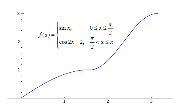
plot(sin(x), x, 0, pi/2)+plot(cos(2*x)+2, x, pi/2, pi)Toggle Line Numbers
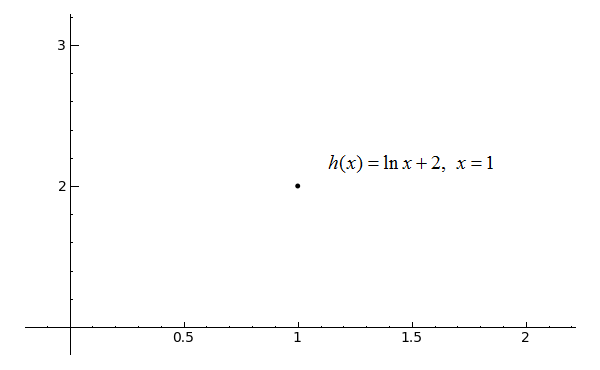
point((1, ln(1)+2), rgbcolor='black').show()Toggle Line Numbers
| · | · | |||||
|
|

|
Tweet | ||||